DAgger Explained

---

Note: All material from this article is adapted from Sergey Levine’s CS294-112 2017/2018 class

Dataset Aggregation, more commonly referred to as DAgger is a relatively simple iterative algorithm that trains a deep deterministic policy solely dependent on the distribution of states of the original and generated dataset. [1]

Here’s a simple example:

Let’s say you’re teaching someone to drive. In this instance, you are a human (hopefully) and your friend’s name is Dave. Despite being a fellow human, Dave’s incapability to drive renders him to be like a policy $\pi_{\theta}(a_t \vert o_t)$. Where $\pi_{\theta}$ is the parameterized policy and $a_t$ is the sampled action space from $o_t$, which is the observation space.

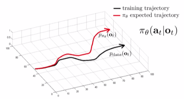
But Dave is smart, beforehand he trained for this exercise by watching some YouTube videos, which we can represent as $p_{data}(o_t)$. Like the rest of us, Dave isn’t perfect and he makes mistakes. In this scenario, however, Dave’s mistakes can quickly add up and result in him (and consequently you) to end up in a ditch or crashing into someone else. We can represent Dave’s distribution for observation as $p_{\pi_{\theta}}(o_t)$. As Dave drives, his mistakes build up, eventually leading him to diverge from $p_{data}(o_t)$, which is the data that Dave trained on (those YouTube videos).

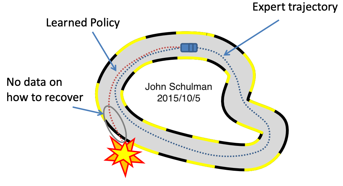
Think of Dave as the red trajectory in the picture. You know that the blue trajectory is correct in your mind and overtime you try to tell Dave to drive like the blue policy.

So how can we help poor Dave? After Dave watches those YouTube videos initially to get some sense of how to drive, he records himself driving. After each episode of driving, we aggregate this data and add in what actions Dave should’ve done to get a new dataset $\mathcal{D_{\pi}}$ which consists of not only $\{o_1,\ldots,o_M\}$ but also the actions corresponding to those observations (since we filled in what actions he should’ve taken for those observations): $\{o_1,a_1,\ldots,a_M,o_M\}$

Now we aggregate the old dataset, $\mathcal{D}$ with this “new” dataset, $\mathcal{D_{\pi}}$ like so: $\mathcal{D} \Leftarrow \mathcal{D} \cup\mathcal{D_{\pi}}$

Surely, you can aggregate the data in whatever way you want, but this is a simple way of doing it.

---

In that example, we essentially implemented DAgger on Dave! Overtime Dave’s distributional mismatch will be nonexistent, meaning Dave will be a driving legend.

Let’s translate the example above to an algorithm:

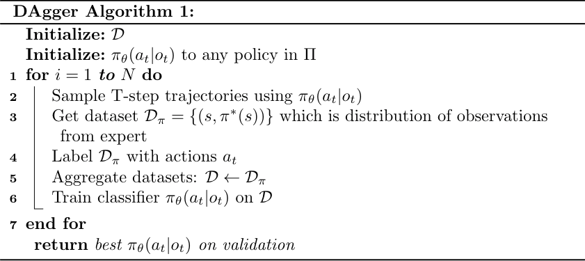
Let’s go through this algorithm step by step:

1. We initialize the dataset $\mathcal{D}$ with initial dataset.

2. Initialize some policy $\pi_{\theta}(a_t \vert o_t)$

3. For N steps (Which is determined by how many times you want to iterate this algorithm. The more times you iterate this algorithm, the better $p_{\pi_{\theta}}(o_t)$ will be like $p_{data}(o_t)$

4. Now inside the for-loop, we sample a trajectory from policy $\pi_{\theta}(a_t \vert o_t)$

5. We get the distribution of observations from $p_{\pi_{\theta}}(o_t)$ which is based on expert dataset, $p_{data}(o_t)$

6. Once we have the distribution of observations, we add in what actions the policy $\pi_{\theta}(a_t \vert o_t)$ should’ve taken

7. We then aggregate the new dataset we have just created with the initial dataset

8. Train classifier $\pi_{\theta}(a_t \vert o_t)$ on this big dataset $\mathcal{D}$

9. Repeat this for loop as long as you want, since $\pi_{\theta}(a_t \vert o_t)$ gets better overtime and asymptotically its $p_{\pi_{\theta}}(o_t)$ will be like $p_{data}(o_t)$

---

Implementation

So how can we implement DAgger in practice?

Well the algorithm is simple enough, so we’ll just need to translate the psuedo-code into Python and for now we won’t go over setup/etc.

This implementation does not require a human. Since DAgger is a Behavior Cloning (BC) algorithm, instead of cloning the behavior of a human, we can just run DAgger against an expert to eventually clone the performance of this expert.

This implementation is based on Jia-Jie Zhu’s Just Another DAgger Implementation. The original repository is unavailable; a preserved copy of the source retains the code and author attribution. [5]

Restoration note — October 2026: Indentation has been restored from that source. These consecutive excerpts retain Python 2 syntax and TensorFlow 1.x/Gym APIs; the source README specifies TensorFlow 1.0.1. They continue inside the same session and DAgger loop and omit the model and environment setup. They are historical examples, not a tutorial for current TensorFlow.

with tf.train.MonitoredSession() as sess:
    sess.run(tf.global_variables_initializer())
    # record return and std for plotting
    save_mean = []
    save_std = []
    save_train_size = []
    # loop for dagger alg

Here we have the initialization for the Tensorflow session we’re starting. Note that I changed the normal tf.Session() to tf.train.MonitoredSession() because it comes with some benefits. Other than that we initialize some arrays we are going to use in the algorithm.

    # loop for dagger alg
    for i_dagger in xrange(50):
        print 'DAgger iteration ', i_dagger
        # train a policy by fitting the MLP
        batch_size = 25
        for step in range(10000):
            batch_i = np.random.randint(0, obs_data.shape[0], size=batch_size)
            train_step.run(feed_dict={x: obs_data[batch_i, ], yhot: act_data[batch_i, ]})
            if (step % 1000 == 0):
                print 'opmization step ', step
                print 'obj value is ', loss_l2.eval(feed_dict={x:obs_data, yhot:act_data})
        print 'Optimization Finished!'

Here we are setting our DAgger algorithm to iterate 50 times. Within the for-loop we start by training our policy $\pi_{\theta}(a_t \vert o_t)$ to fit the MLP, which stands for Multilayer Perceptron. It’s essentially a standard feedforward NN with an input, hidden, and output layer (very simple).

To put this step in other words, given this is the 1st iteration, Dave from the earlier example has just gotten some idea on how to drive by watching those YouTube videos. In later iterations, Dave, $\pi_{\theta}(a_t \vert o_t)$ is essentially training on the entire dataset $\mathcal{D}$. This is out-of-order, but this is step 6 in our algorithm. It doesn’t matter though since all parts of the algorithm are incorporated in this implementation, in order.

        # use trained MLP to perform
        max_steps = env.spec.timestep_limit
        returns = []
        observations = []
        actions = []
        for i in range(num_rollouts):
            print('iter', i)
            obs = env.reset()
            done = False
            totalr = 0.
            steps = 0
            while not done:
                action = yhat.eval(feed_dict={x:obs[None, :]})
                observations.append(obs)
                actions.append(action)
                obs, r, done, _ = env.step(action)
                totalr += r
                steps += 1
                if render:
                    env.render()
                if steps % 100 == 0: print("%i/%i" % (steps, max_steps))
                if steps >= max_steps:
                    break
            returns.append(totalr)
        print('mean return', np.mean(returns))
        print('std of return', np.std(returns))

Here, we are rolling out our policy Dave (in other words $\pi_{\theta}(a_t \vert o_t)$). What does policy rollout mean?

Does it have something to do with a roly poly rolling out? As you could guess, it doesn’t. Rather, it’s essentially our policy exploring trajectories, eventually building up a distribution of $p_{data}(o_t)$. This is steps 2 and 3 in our algorithm.

        # expert labeling
        act_new = []
        for i_label in xrange(len(observations)):
            act_new.append(policy_fn(observations[i_label][None, :]))
        # record training size
        train_size = obs_data.shape[0]
        # data aggregation
        obs_data = np.concatenate((obs_data, np.array(observations)), axis=0)
        act_data = np.concatenate((act_data, np.squeeze(np.array(act_new))), axis=0)
        # record mean return & std
        save_mean = np.append(save_mean, np.mean(returns))
        save_std = np.append(save_std, np.std(returns))
        save_train_size = np.append(save_train_size, train_size)
dagger_results = {'means': save_mean, 'stds': save_std, 'train_size': save_train_size,
                  'expert_mean':save_expert_mean, 'expert_std':save_expert_std}
print 'DAgger iterations finished!'

We have the last process necessary for DAgger here. Here we expertly label the distribution of $p_{data}(o_t)$ with our expert policy. This is steps 4 and 5 in our algorithm.

Wasn’t that fun? Hopefully you get a better idea of what DAgger is. You can find the code by Jia-Jie Zhu in the preserved repository. If you have any problems, feel free to contact me at surya@suryad.com

---

References

[1] A Reduction of Imitation Learning and Structured Prediction to No-Regret Online Learning, Ross, Gordon & Bagnell (2010). DAGGER algorithm [link]

[2] Deep DAgger Imitation Learning for Indoor Scene Navigation [PDF]

[3] DAGGER and Friends [PDF]

Schulman, J., 2015.

[4] CS294-112 Fa18 8/24/18 [link]

Levine, S., 2018.

[5] Just Another DAgger Implementation, preserved source.

Zhu, J.J., 2017. MIT license.